Classification of Handwritten digits with Tensorflow
Recently, I took up NVIDIA’s course on Machine Learning with the Jetson Nano - a short four hour course that gives you an introduction to machine learning using the Jetson Nano and Python. As a part of the course, I created a short project to classify handwritten digits using Tensorflow, Convolutional Neural Networks and the MNIST database.
What is a Convolutional Neural Network (CNN)?
In deep learning a CNN is a class of an artificial neural network. The name comes from ‘convolution’ - the mathematical operation on two functions that expresses how the shape of one function modifies the other. A convolution neural network refers to an operation where the process of convolution is used at least once in place of multiplying two matrices.
Each layer of a CNN consists of many nodes or neurons. Similar to the neurons in our brain, a neuron in machine learning refers to something that takes in an input, processes it and returns an output for the next neuron to process. Each neuron is provided a set of conditions called a bias and if the input satisfies this set, the neuron performs its task and returns an output. This bias is the same for all neurons in that layer.
The inputs also come with a set of values that factor into each neuron’s output called a weight. The weight of an input defines the input’s importance to the neuron. For example, say that you’re deciding between three drinks and you prefer drinks with ice in them regardless of the flavour. So the presence of ice factors in more to the decision you finally make compared to the flavour of the drink, which results in the ice having a higher weightage in the decision making process.
Finally, to make the neuron’s calculations easier, a function is created to limit the range of inputs. If the inputs vary a lot in value, an activation function is used to transform the given set of inputs to range between two values known to the CNN. For example, if the inputs vary between -3 and 200, a sigmoid activation function (a particular type of activation function) transforms this range to make it fit between 0 and 1. For this project, I used the ReLU activation function that returns the input if the value is positive and returns a zero if it is negative. It has become the default activation function because it’s easy to train and achieves better performance.
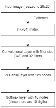
In order to classify the handwritten digit, a CNN is created and a set of instructions is given to it to classify in the input image into given categories. When the i mage of the handwritten digit is given as input to the model in the form of a matrix, it goes through multiple layers of mathematical operations and is compared with the set of instructions provided. The image is fed into the CNN in the form of a tensor. At the end of the network, the image is classified into one of ten categories (each representing a digit).

First the image is resized to 28 x 28 pixels, then flattnened into a matrix of dimensions 1 x 784 so that the CNN can process the image. The flattened image is put through a convolution layer which provides the important features of the image to the next layer. The second and third layers are dense layers with 128 neurons. Finally the processed data is classified into one of ten nodes, each node representing one digit, in the last layer.
The Code Explained
Loading the Data
mnist = tf.keras.datasets.mnist
(x_train, y_train),(x_test, y_test) = mnist.load_data()
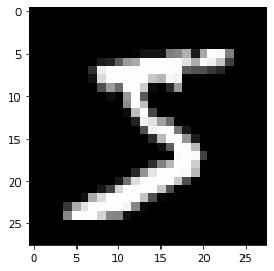
First I load the MNIST dataset using Tensorflow. Here’s an example of what is in this set.

Preparing the data for the model
The values of each image is then scaled from its default range of 0 to 255 to a range of 0 to 1 so that the CNN can process the data easier.
xTrain = tf.keras.utils.normalize(x_train, axis=1) # normalizing training data
xTest = tf.keras.utils.normalize(x_test, axis=1) # normalizing testing data
Creating the model
Now using the Sequential() function in Tensorflow, the CNN is created.
model = tf.keras.models.Sequential()
model.add(tf.keras.layers.Flatten())
model.add(tf.keras.layers.Dense(128, activation=tf.nn.relu)) # CNN Layer 1
model.add(tf.keras.layers.Dense(128, activation=tf.nn.relu)) # CNN Layer 2
model.add(tf.keras.layers.Dense(10, activation=tf.nn.softmax)) # CNN Final Layer
The model is then compiled and then fitted according to the training data. The function model.fit() arranges the training data to correspond to the labels associated with that data. For example, the training data that consists of a handwritten seven is associated with the label ‘7’.
# model compiles here
model.compile(optimizer="adam",
loss="sparse_categorical_crossentropy",
metrics=["accuracy"])
# model if fitted here
model.fit(x=xTrain, y=y_train, epochs=5) # model fitted
This process runs multiple times and each time the weights and outputs are adjusted slightly to increase the model’s accuracy. Each iteration is called an ‘epoch’. Here’s the result for running the function with five epochs.
Epoch 1/5
1875/1875 [==============================] - 3s 1ms/step - loss: 0.2601 - accuracy: 0.9228
Epoch 2/5
1875/1875 [==============================] - 3s 1ms/step - loss: 0.1062 - accuracy: 0.9668
Epoch 3/5
1875/1875 [==============================] - 2s 1ms/step - loss: 0.0718 - accuracy: 0.9772
Epoch 4/5
1875/1875 [==============================] - 2s 1ms/step - loss: 0.0520 - accuracy: 0.9830
Epoch 5/5
1875/1875 [==============================] - 2s 1ms/step - loss: 0.0405 - accuracy: 0.9871
Testing the model
The model can be tested using the predict() function. It takes in a tensor of dimensions (n, 28, 28) where n represents the number of images in the dataset. The function’s output is an array of values and the index of its maximum value represents the model’s prediction.
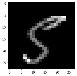
For this test I’m using the following image from the training data:
plt.imshow(xTest[211], cmap='gray')
plt.show()

prediction = model.predict([xTest])
print(prediction = model.predict([xTest])) # prints the model's prediction
Integration of OpenCV to detect handwritten digits live
Now that the model works, it’s time to integrate some computer vision into the project.
# this function is used as a callback function for the trackbar created
def nothing(x):
    pass

cv2.namedWindow('frame')
cv2.createTrackbar('r', 'frame', 0, 255, nothing)
cv2.setTrackbarPos('r', 'frame', 23)
cap = cv2.VideoCapture(0)
currentVal = 0
modelOut = 0

# creating an empty dataset that can hold five images at a time
inData = np.empty((5, 28, 28))
inData is a tensor created so that the model can run on the code every five frames.
while True:
    if currentVal == 4:
        prediction = model.predict([inData])
        modelOut = np.argmax(prediction[currentVal-2])

        inData = np.empty((5, 28, 28))
        currentVal = 0
This section runs the model on the set of frames collected every five frames. modelOut is then displayed on the program’s output window.
    ret, frame = cap.read()
    gray = cv2.cvtColor(frame, cv2.COLOR_BGR2GRAY)
    threshold = int(cv2.getTrackbarPos('r', 'frame'))
    _, thr = cv2.threshold(gray, threshold, 255, cv2.THRESH_BINARY_INV)
In this section, the live camera feed is first converted to grayscale, then to an image where all color values are transformed to either be 0 or 1. The threshold beyond which the value is transformed to a 1 is determined by the user using the trackbar on the output window.
    h = 200
    w = 200
    y = int((frame.shape[0]/2)-h/2)
    x = int((frame.shape[1]/2)-w/2)

    cv2.rectangle(frame, (x, y), (x + w, y + h), (255, 0, 0), 2)
    area = thr[y:y+w, x:x+w]
    area = cv2.resize(area, (28, 28))
A rectangle is drawn on the output window and an area of size 200 x 200 pixels is associated with the variable area. This area is then resized to an image of 28 x 28 pixels so it can be fed into the created model.
    areaFlattened = tf.keras.utils.normalize(area, axis=1)
    inData[currentVal] = areaFlattened
    cv2.putText(frame, str(modelOut), (30, 30),
        cv2.FONT_HERSHEY_COMPLEX, 1, (255, 0, 0),
        1, cv2.LINE_AA, False)
area is then flattened so that all its values range from 0 to 1. Each frame of area is then added to inData and the model’s output is displayed on the output window. The output
    cv2.imshow('thr', thr)
    cv2.imshow('frame', frame)
    currentVal += 1
    if cv2.waitKey(20) & 0xff == ord('q'):
        cv2.imwrite('area.png', area)
        break
The output window(frame) and thresholded image(thr) are displayed. A condition is created for the loop to break if the ‘q’ key is pressed.
Here’s a short demonstration of the project working.
Conclusion
This is the first of hopefully many machine learning projects. I had a lot of fun making this and managed to learn about many new concepts in mathematics. Hopefully you liked this article.
That’s all I have for now. Live long and prosper!
Resources
GitHub Repository - Download the code and run main.ipynb.
Dependencies:
- OpenCV (v4.5+)
- Tensorflow (v2.6+)
- Numpy (v1.20+)
- Matplotlib (v3.4+)