Python Playground: OpenGL!
In October 2022, I started reading Python Playground and wrote an article to mark the day I started.
As of today, I finished reading and coding for the eighth, ninth and tenth chapters of Python Playground - the introduction of and experimentation with OpenGL. OpenGL is an API that allows fast and efficient rendering. It operates on a C-like shading language (GLSL) to write shaders.
Projection and Modelview Matrices
In OpenGL, Projection matrices are used to project the 3D object into the 2D image seen on screen. Modelview matrices are used to position 3D objects in the space. These transformation matrices are applied to homogenous coordinates represented by (x, y, z, w) which is equivalent to (x/w, y/w, z/w, 1.0).
A set of homogeneous coordinates (x, y, z, 1.0) can be translated to another point (x+t, y+t, z+t, 1.0) through the following operation.

Vertex Shaders
A vertex shader is a graphics processing function that handles processing of induvidual verticies. In Chapter 9, the first vertex shader defined is a simple shader that adds a vertex aVert with a color.
#version 330 core
v in vec3 aVert;
w uniform mat4 uMVMatrix;
x uniform mat4 uPMatrix;
y out vec4 vCol;
void main() {
    // apply transformations
    z gl_Position = uPMatrix * uMVMatrix * vec4(aVert, 1.0);
    // set color
    { vCol = vec4(1.0, 0.0, 0.0, 1.0);
}
Fragment Shaders
A fragment shader helps render the set of verticies generated by the vertex shader into the render window. The following fragment shader sets the input fragment’s color based on input vCol.
#version 330 core
v in vec4 vCol;
w out vec4 fragColor;
void main() {
    // use vertex color
    x fragColor = vCol;
}
The fragment shader is executed for every pixel on screen while the vertex shader defines every vector in the scene regardless of whether or not it is being viewed.
Both fragment and vertex shaders are written in GLSL and then loaded into Python.
Vertex Buffers
In order to efficiently draw 3D geometry, a Vertex Array Object (VAO) is created to store arrays of coordinates, colors and attributes. Vertex Buffer Objects (VBOs) are created for each attribute and defined at every vertex. The location of VAOs in the shader are specified and enabled. The data is then ready to render. VBOs store the vertex data in the GPU.
Chapter 9: Simple Texture Rendering
Chapter 9 involves the rendering of a square with a pre-defined star texture rendered onto it.
Vertex shader:
#version 330 core

layout(location = 0) in vec3 aVert;

uniform mat4 uMVMatrix;
uniform mat4 uPMatrix;
uniform float uTheta;

out vec2 vTexCoord;

void main() {
  // rotational transform
  mat4 rot =  mat4(
		vec4( cos(uTheta),  sin(uTheta), 0.0, 0.0),
		vec4(-sin(uTheta),  cos(uTheta), 0.0, 0.0),
	    vec4(0.0,         0.0,         1.0, 0.0),
	    vec4(0.0,         0.0,         0.0, 1.0)
	    );
  // transform vertex
  gl_Position = uPMatrix * uMVMatrix * rot * vec4(aVert, 1.0);
  // set texture coord
  vTexCoord = aVert.xy + vec2(0.5, 0.5);
}
The rotational matrix slowly rotates the set of shapes based on uTheta.
def step(self):
    # increment angle
    u self.t = (self.t + 1) % 360
    # set shader angle in radians
    v glUniform1f(glGetUniformLocation(self.program, 'uTheta'),
    math.radians(self.t))
The step function increments the angle by 1 and calls the vertex shader to rotate the texture.
Fragment shader:
#version 330 core

in vec2 vTexCoord;

uniform sampler2D tex2D;
uniform bool showCircle;

out vec4 fragColor;

void main() {

    #define PI 3.1415926535897932384626433832795

    if (showCircle) {
        if (sin(16*PI*distance(vTexCoord, vec2(0.5, 0.5))) < 0.0) {
            discard;
        }
        else {
            fragColor = texture(tex2D, vTexCoord);
        }
    }
}
The fragment shader allows the rendering of several concentric circles on top of the rotating texture.
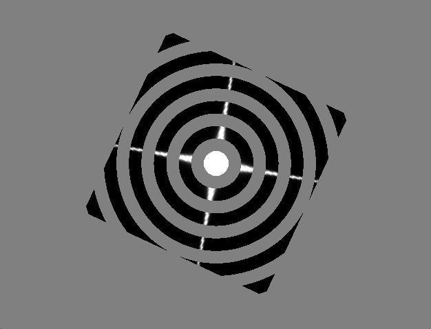
Code to the chapter is available here.
Chapter 10: A Fountain of Particles
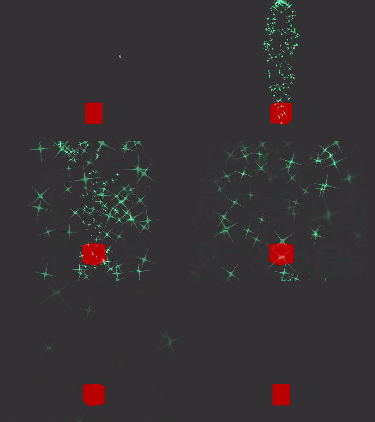
Chapter 10 involves the creation of particle systems based on certain conditions. The program simulates particles flying upwards in a fountain-like arc. The motion of each particle is modeled by the following equation.
$P = P_{0} + V_{0}t + \frac{1}{2}at^{2}$
To limit the distribution of particles, the particles are directed along a narrow region of 20 degrees of inclination from the Z-axis. The angle at which the particle is directed vertically is $\theta$. The angle at which the particle is directed horizontally is $\phi$.
$\theta = random([0, 20])$
$\phi = random([0, 360])$
To ensure the particles don’t rise at the same time, a short time delay of 0.05 seconds is added between each particle’s launch.
Each particle is textured similar to how Chapter 9 rendered a star texture onto a square, however the particles are blended into the environment by setting the black regions of the star texture to transparent. Finally, to ensure that all the sparks face the camera, a technique call bill-boarding is used.
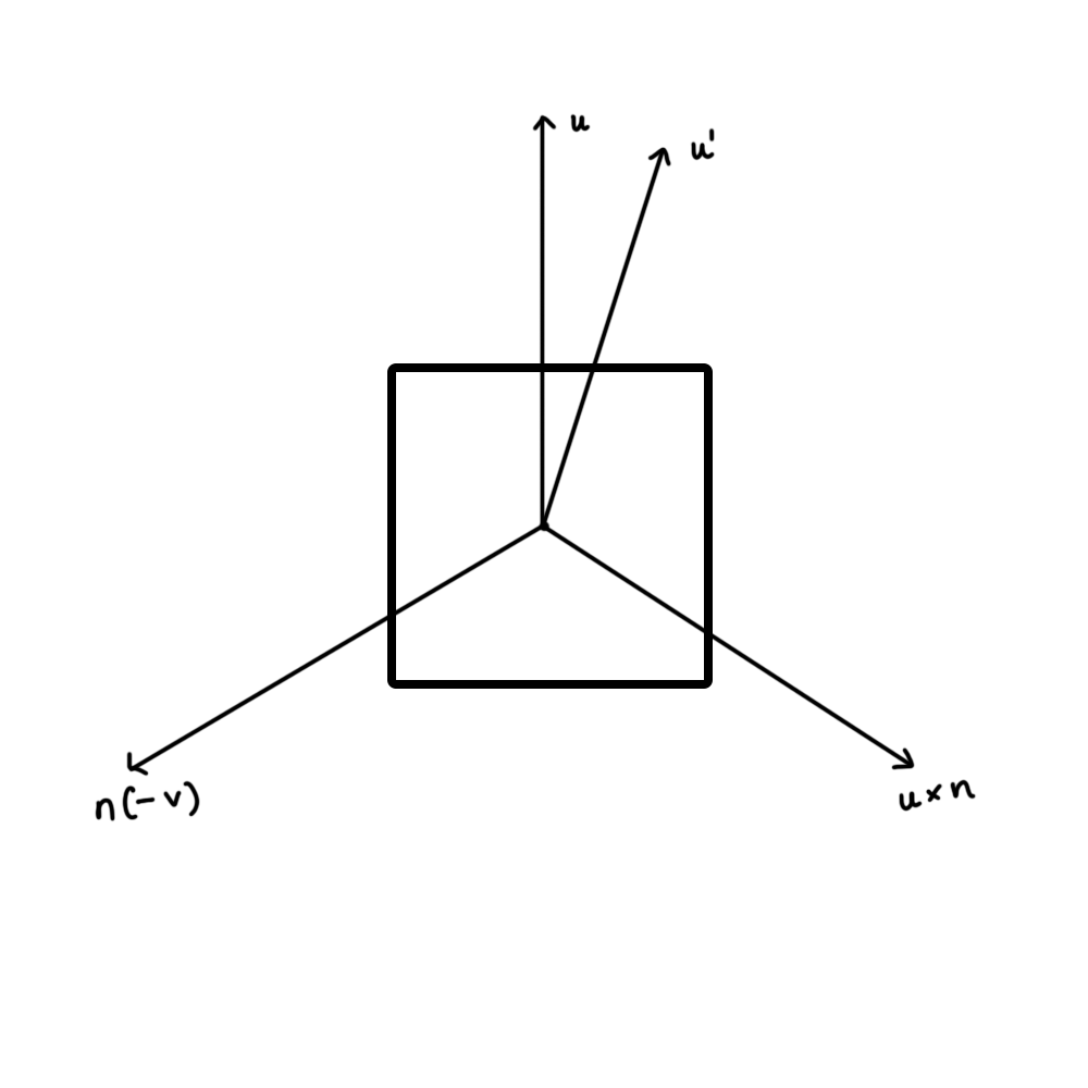
Billboarding faces the normal vector (n) of the quad towards the camera. Vector u represents the up vector for the final orientation of the quad given by (0, 0, 1). Then vector $r = u \times n$ is calculated which is mutually perpendicular to n and u. A third vector $u’ = n \times r$ is calculated. The three vectors (r, u’ and n) are orthogonal. The vectors are normalized and then rotated based on the following matrix.

Vertex shader:
#version 330 core

in vec3 aVel;
in vec3 aVert;
in float aTime0;
in vec2 aTexCoord;

uniform mat4 uMVMatrix;
uniform mat4 uPMatrix;
uniform mat4 bMatrix;
uniform float uTime;
uniform float uLifeTime;
uniform vec4 uColor;
uniform vec3 uPos;

out vec4 vCol;
out vec2 vTexCoord;

void main() {
    float dt = uTime - aTime0;
    float alpha = clamp(1.0 - 2.0*dt/uLifeTime, 0.0, 1.0);
    if(dt < 0.0 || dt > uLifeTime || alpha < 0.01) {
        gl_Position = vec4(0.0, 0.0, -1000.0, 1.0);
    }
    else {
        vec3 accel = vec3(0.0, 0.0, -9.8);
        float PI = 3.14159265358979323846264;
        float theta = mod(100.0*length(aVel)*dt, 360.0)*PI/180.0;
        mat4 rot = mat4(vec4(cos(theta), sin(theta), 0.0, 0.0),
                vec4(-sin(theta), cos(theta), 0.0, 0.0),
                vec4(0.0, 0.0, 1.0, 0.0),
                vec4(0.0, 0.0, 0.0, 1.0));

        mat4 sc = mat4(vec4(dt*2.0, 0.0, 0.0, 0.0),
                    vec4(0.0, dt*2.0, 0.0, 0.0),
                    vec4(0.0, 0.0, dt*2.0, 0.0),
                    vec4(0.0, 0.0, 0.0, 1.0));
        vec4 pos2 = bMatrix*rot*vec4(aVert, 1.0)*sc;

        if (pos2[2] == 0.0) {
            pos2 = pos2 * 10.0;
        }
        vec3 newPos = pos2.xyz + uPos + aVel*dt + 0.5*accel*dt*dt;
        gl_Position = uPMatrix * uMVMatrix * vec4(newPos, 1.0);
    }
    vCol = vec4(uColor.rgb, alpha);
    vTexCoord = aTexCoord;
}
Fragment shader:
#version 330 core
uniform sampler2D uSampler;
in vec4 vCol;
in vec2 vTexCoord;
out vec4 fragColor;
void main() {
    vec4 texCol = texture(uSampler, vec2(vTexCoord.s, vTexCoord.t));
    fragColor = vec4(texCol.rgb*vCol.rgb, vCol.a);
}
Output:
Chapter 11: Volume Rendering
This was a tough cookie to crack.
Volume rendering is a technique used to construct 3D images. MRI and CT scans often use this technique to render a 3D volume from cross-section 2D images. The volume is created using ray-casting - a method by which a ray is shot into a 3D volumetric dataset for every pixel in the 2D image. The data is sampled at regular intervals along the 3D dataset (usually represented as a cube) to compute the final intensity of the image.
MRIs and CT scans often use this technique to render a 3D volume from a set of 2D images or slices.
Rays are generated per-pixel through a unit cube whose color at any given point is represented by the coordinates of that point.
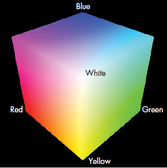
Each ray is represented by a vector R in the volume cube. First the back-faces of the cube are drawn into an FBO (Frame Buffer Object). The ray is computed by subtracting the front-face color of the fragment being rendered from the back-face color which is read from the texture of the 2D image.
#version 330 core

in vec4 vColor;

uniform sampler2D texBackFaces;
uniform sampler3D texVolume;
uniform vec2 uWinDims;

out vec4 fragColor;

void main()
{
    // start of ray
    vec3 start = vColor.rgb;

    // calculate texture coords at fragment, which is a
    // fraction of window coords
    vec2 texc = gl_FragCoord.xy/uWinDims.xy;

    // get end of ray = back-face color
    vec3 end = texture(texBackFaces, texc).rgb;

    // calculate ray direction
    vec3 dir = end - start;

    // normalized ray direction
    vec3 norm_dir = normalize(dir);

    // the length from front to back is calculated and
    // used to terminate the ray
    float len = length(dir.xyz);

    // ray step size
    float stepSize = 0.01;

    // X-Ray projection
    vec4 dst = vec4(0.0);

    // step through the ray
    for(float t = 0.0; t < len; t += stepSize) {

        // set position to end point of ray
        vec3 samplePos = start + t*norm_dir;

        // get texture value at position
        float val = texture(texVolume, samplePos).r;
        vec4 src = vec4(val);

        // set opacity
        src.a *= 0.1;
        src.rgb *= src.a;

        // blend with previous value
        dst = (1.0 - dst.a)*src + dst;

        // exit loop when alpha exceeds threshold
        if(dst.a >= 0.95)
            break;
    }

    // set fragment color
    fragColor =  dst;
}
The ray is computed by normalizing the vector found by subtracting the front-face point from the back-face point. The program then iterates through every point on the ray and gets the texture value at each position. It then sets the opacity of the volume at that point based on the texture provided by the 2D image slice.
I used the same dataset as the book for this example which can be found here.
Output:
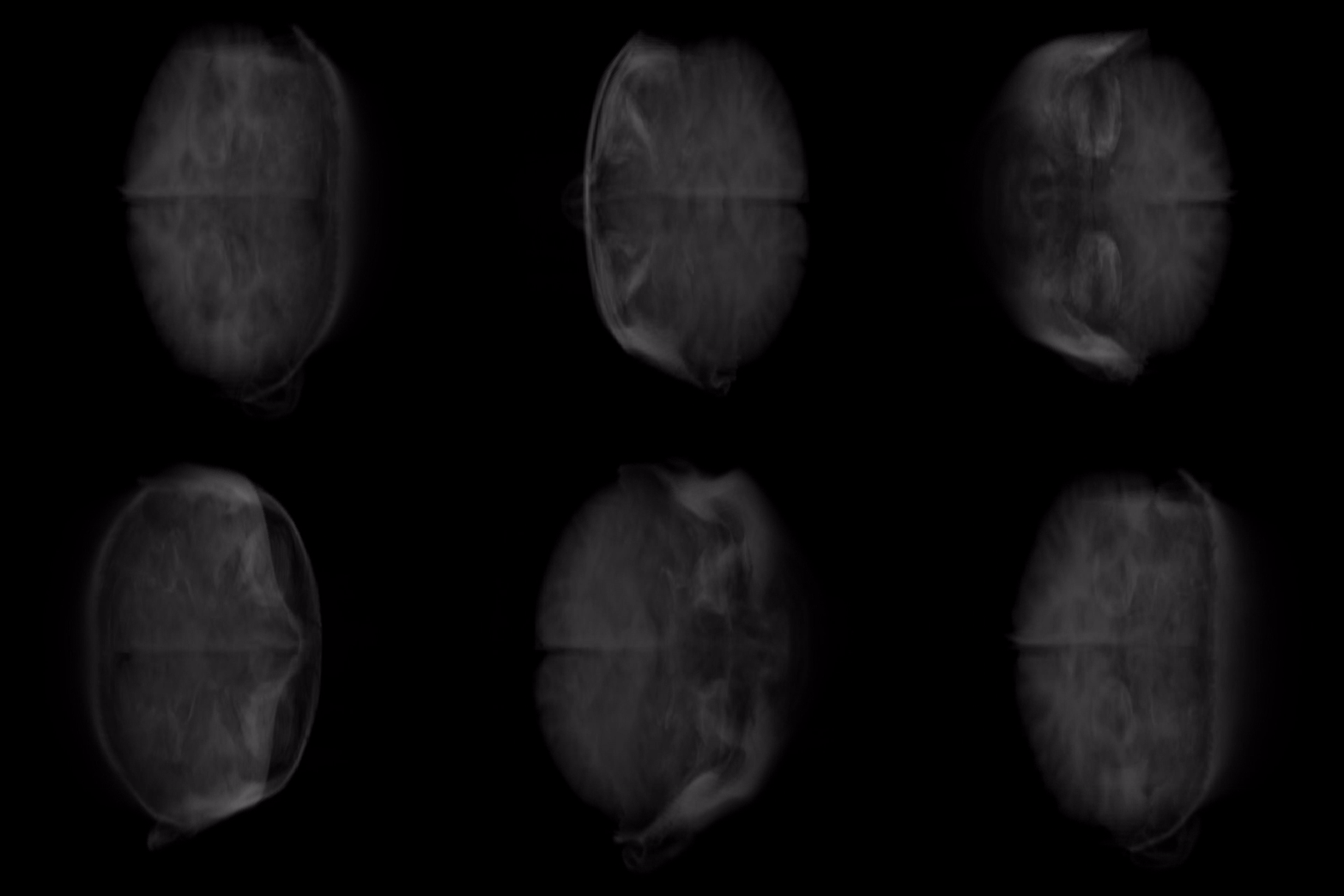
Here’s what the final volume looks like-
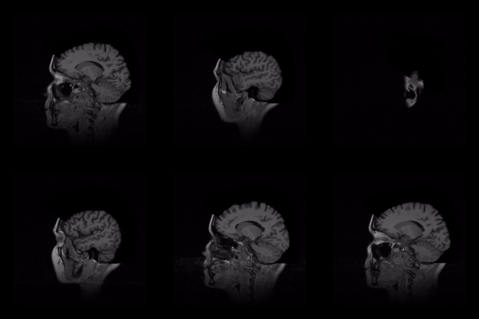
Here’s a quick cycle through the 2D slices that created the final volume.
Summary
OpenGL is a fascinating topic to me. I’ve combined the three chapters into this article both because of how interconnected they are conceptually and because it serves as references for my future self in case I need to remember an explanation I can better understand. Compiling this article has only made me understand it better but… it is not a simple topic. Even now, I’m attempting to understand the pieces of code I’ve written.
That’s all I have for now. Live long and prosper.